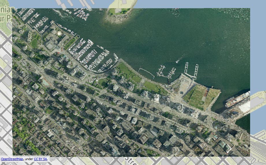
Are you ready to go on a crash course about spatial data and how it all works together? Buckle up because we are about to get the facts straight about integrating the geometry models known as vector and raster data. Of course, we’re going to cover the basics of vector and raster along the way, and wrap up by talking about the challenges and key considerations when transforming between raster (JPEG, GeoTIFF, etc.) and vector (shapefile, KML, etc.) formats.
Feel free to jump to the transforming section if you are already familiar with vector and raster geometry types.
Alright, here we go…
What is Vector Data
Vector data features are most commonly represented as point(s), line(s), or polygons(s). While these may be the most common vector types, they are not the only ones! There are also more complex vector geometry types like donuts, arcs, and even curvy things called clothoids. And that’s just covering 2D geometry. If your data has a z coordinate with every coordinate pair, you have an entirely new set of geometries to account for. But for the sake of this article, let’s keep it simple and stick with the three basic 2D geometries.
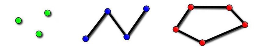
- Points: a single set of X/Y coordinates.
- Lines: a series of connected points that form a chain.
- Polygons: a series of connected points whose first and last points are the same to form an enclosed shape.
That’s right! These three basic geometries, likely the same ones you likely learned about in school as a kid, are the most commonly used spatial geometries.
Points represent individual assets like a bus stop, an address point (like your favourite restaurant), or a street light. Lines represent linear objects that make up a network, like power lines, road centerlines, or even water lines where each node or connection is a vertex on the line. Polygons represent a boundary like a building outline or territorial boundaries for things like parcels, cities, states, etc.
As shown in the image above, the actual shape these features depict is handled by the number of vertices (set of X/Y Coordinates). A line or polygon with many vertices will appear less jagged than an equivalent shape with fewer vertices.
Alright, that covers the basics of vector geometry, let’s square things up and talk about rasters.
What is Raster Data
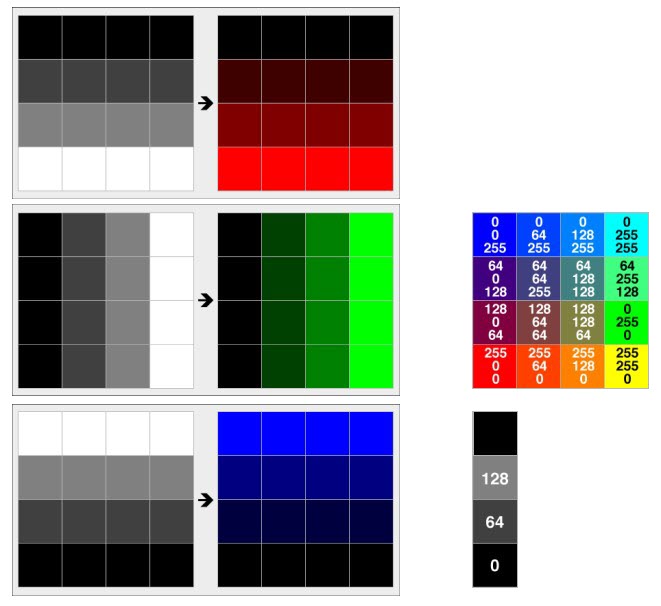
Like vector geometry, raster geometry is quite simple. It’s uniform in nature and follows a grid of cells organized by columns and rows. Raster data starts to get complex when you look at an individual cell with numeric or color values (like an image you take on with your phone). The values of the cell depends on the sensor (or in the case of an image on your phone, the camera sensor) used to record the data, which may have multiple channels to record even more information about each cell! This is typically the case for LiDAR and aerial imagery where cameras and sensors record everything from color, temperature, elevation, and other qualitative information.
Raster: a grid of values organized into rows and columns. Each row and column intersection in the grid is called a cell or pixel.
Raster data may appear simple, but can be quite complex in nature. For the sake of teaching, we’ll stick to a simple example of colour rasters to explain how rasters work. Color rasters are typically derived from satellite data or imagery that records data in 3 channels: red (R), green (G), and blue (B). Each channel also records a brightness value which so that when all three channels are overlaid onto the same grid they display unique colours we see.
Transforming Between Geometry Models
Rasterization (Vector to Raster)
Ok now let’s consider transforming from one geometry model type to another. Of course, it’s easy to start with a point and add another vertex in order to create a line. And, you guessed it, add one more vertex and you get a polygon feature.
But, when we want to transform a vector feature into a raster feature, there are several key considerations to make:
- What are your resolution/file size specifications (i.e. columns, rows, cell spacing):
- Will you be compressing or tiling your output to reduce file size an improve loading times
- Does your destination format support an alpha band
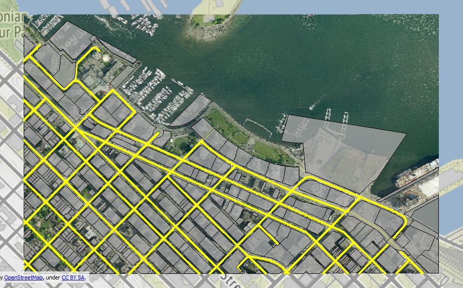
Each geometry type has benefits and disadvantages because they are built for specific purposes. However, depending on what you are trying to accomplish with your dataset, it might be necessary to convert between raster and vector geometry.
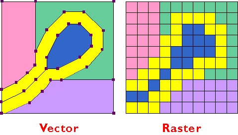
In the example above, the edges of the vector polygons are represented as entire cells when converted to raster.
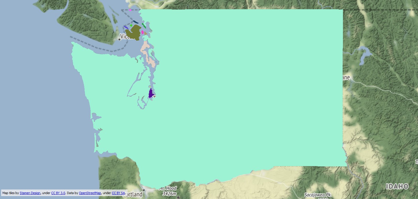
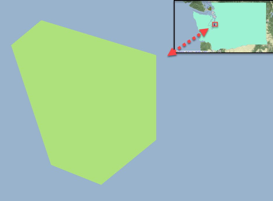
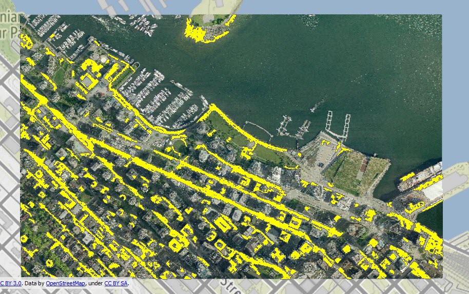
The example above is simple, however, in reality your output may look something like this:
Vector

Raster
Easy to tell the difference, right? Well… maybe not from this extent, but let’s zoom in and take a closer look.
Vector
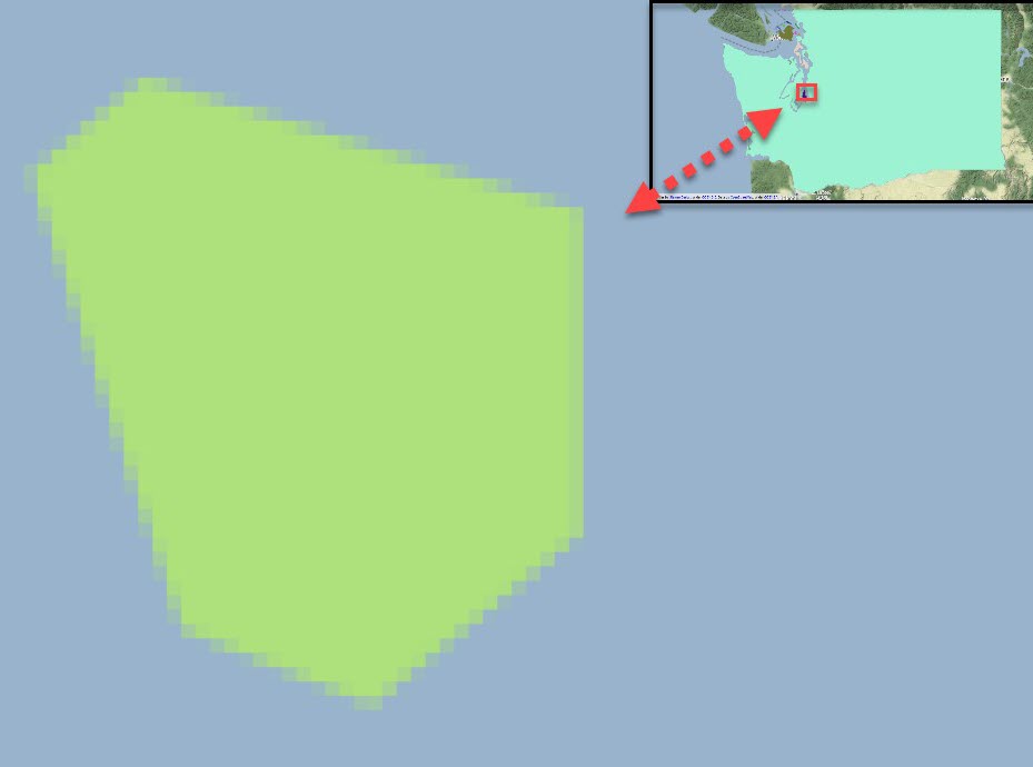
Raster
Ahh much better. Now you can really see the difference between a vector dataset that was converted to a raster dataset with 100m cell size.
Even with this basic polygon, you can clearly see that some cells in the raster are fully contained within the vector polygon (pixel 4 in the image below) while others only have a partial overlap (pixels 1-3). As a result of the varying degree of overlap, our transformation has produced cells that have a smooth gradient from areas with 100% overlap, to areas that have <100% overlap with the specified cell size.
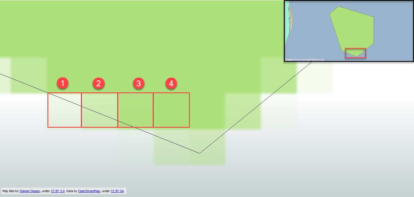
This is an example of a “fuzzy” result. It’s considered “fuzzy” because the pixels values make up various shades of green. As you can see in the screenshot above, the areas with the greatest overlap produced the darkest green, whereas the areas with lower overlap are represented by a lighter shade of green. However, raster datasets can also follow boolean logic like the screenshot below, where cells are coloured identically no matter what level of overlap there is (although this is less common among raster datasets).
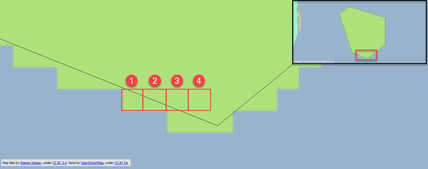
As you can tell, when transforming data from vector to raster, straight lines can end up looking more like a staircase. How coarse or fine the staircase ends up being is dependent on the resolution or cell size you end up using when rasterizing your data.
One of the more common use cases for rasterizing vector data is for map production. This is something that can easily be accomplished and reproduced in FME using a single transformer called the MapnikRasterizer, but that is just one way to convert vector data to raster!
Vectorization (Raster to Vector)
You may have had a raster dataset come across your desk and need to extract features from the dataset and produce a series of vector datasets. Perhaps you want to create contour lines from a DEM file or extract roads/buildings from a raster dataset. Depending on the task, there are several approaches you can take to extract the features of interest.
Let’s take a look at a 1m GeoTIFF file and extract roads and buildings using a cell value extraction approach. Extracting features by cell values enables you to define a range of acceptable cell values to convert to a vector feature. This can be a bit of a balancing act because you want the range to be inclusive enough to find as many features of interest as possible. At the same time, this range should be exclusive in order to prevent unwanted features from creeping into the results. In the example below, the cell values of interest are grey which happen to have cell values that fall between 100-160 for each band (R, G, B).
Source
Expectation
Reality
Considering the resolution of the source dataset, this isn’t a bad starting point. We’ve been able to extract a good portion of the roads purely based on cell values that make up the grey color of the cement. However, this method isn’t foolproof as the extracted roads will need to be cleaned up and QA’d further to ensure the results are accurate. If we had a higher resolution image, we could try to extract the yellow stripe in the middle of the roads – this goes to show how cell size can drastically improve/degrade the output vector feature(s).
How can we improve the results? Perhaps we could leverage a computer vision workflow using a RasterObjectDetector or connecting to Picterra to improve the accuracy. Or by tracing the raster dataset using Potrace. Regardless of your approach, one thing to keep in mind with vectorization is that while you can automate feature extraction, in some cases you may only be able automate a portion of the process and the rest needs to be manually extracted by digitizing. It is always a good idea to QA your data for accuracy and ensure no false negatives/positives make their way into your output.
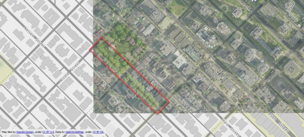
For example, you can see in the bottom left corner of the GeoTIFF, we’re missing some sections of road due to tree canopy coverage. Regardless of the feature extraction method you use (i.e. extract by cell values, computer vision, etc), areas like this will need to be manually digitized.
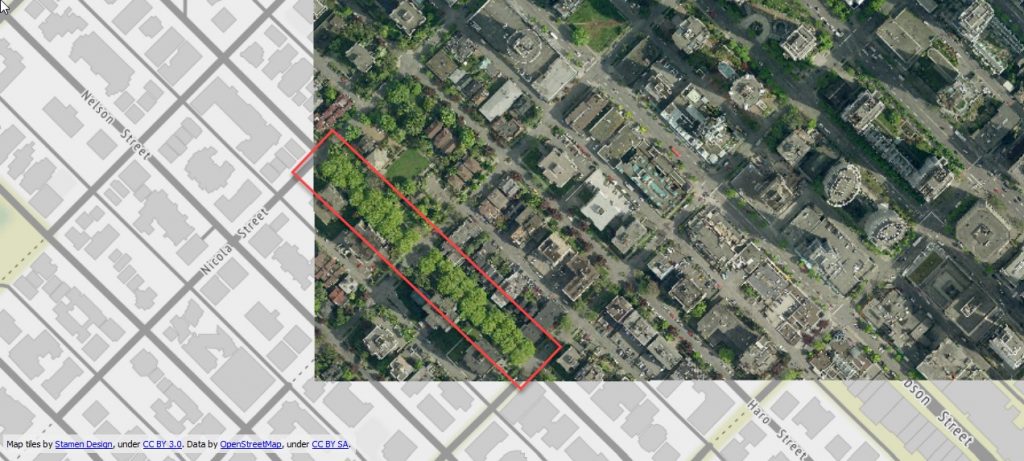
While this tree coverage may look like a park or a greenbelt, it is in fact a section of road called Barclay Street which we can see by increasing the transparency of the dataset and overlaying it on top of a basemap in the FME Data Inspector.
Don’t get me wrong, this article isn’t meant to say feature extraction can’t be fully automated. It certainly can be, but the quality of the output is entirely dependent on the quality of the source data (cell size, shadows, cloud/canopy coverage, etc.). As with anything, garbage in = garbage out. This applies to both the source dataset, as well as the model used for object detection.
Integrating Vector and Raster Data
We have to talk about the third sphere of working with raster and vector data. You could be working with a variety of formats with different schemas, coordinate systems, and as we’ve already seen, geometry types. But, that doesn’t mean you’re limited to working only with 1 geometry model in your workflow.
Other methods of rasterization include vector on raster overlay which allows you to make an imprint of the vector geometry on top of a raster dataset. Alternatively, both raster and vector datasets can be used in the same workflow for things like clipping your data to the desired extents. Even on the 3D side of things, vector features can be draped over 3D surfaces, raster datasets can be used as appearances to provide more context about the feature!
Other Considerations
Before you start your journey with converting data from raster to vector or vector to raster, one of the most important considerations to keep in mind is whether your desired output format supports that geometry type. Not all formats are created equally. Some support only certain types of vectors and certain raster formats require a certain band interpretations to be set. Some formats even support both geometry types! I’m looking at you PDF & KML…
Regardless of the format, geometry support specifications are listed in the Quick Facts section of every FME Writer Documentation page but we are always happy to help in the Community Forum or on Live Chat if you even need a second opinion or are feeling a little lost.
Ever wonder how FME could be utilized in your organization? Request a personalized Product Demo to chat directly with our team about your use case and how FME can help! Or check out our live demos gallery to see some examples of FME in action!
You might also want to read:
Integrating Third-Party Tools with FME (No Coding Required)

Christian Berger
Chris is one of the FME Desktop Technology Experts that helps users in their day to day data issues. He’s not just a GIS buff though - he also used to play on his university’s football team!