About six years ago, we added point clouds as a new member of the FME geometry family. Since that time, many of our customers have used FME point cloud tools for all kinds of operations on data consisting mostly of LiDAR scans.
From the most popular scenario of surface generation, to urban scene visualization, vegetation growth control, and road quality assessment, our users usually deal with point clouds in their traditional form and for well-established purposes.
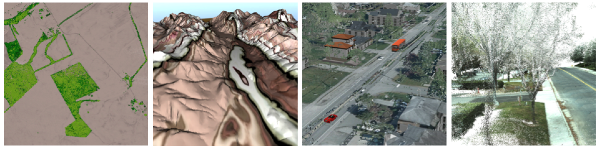
Typical uses of point clouds.
But point clouds can play unusual roles in scenarios where traditionally we wouldn’t see a place for them.
Advantages of Using Point Clouds
Why should we even think about using point clouds outside of their traditional areas? Well, here is the main answer: point cloud processing is extremely efficient when dealing with huge data volumes.
How FME Processes Point Clouds So Effectively
Here is a simple example: if we read a text file with over 3,000,000 XYZ coordinates point by point, it takes 2.5 minutes. If we read the same file as a point cloud, it takes less than 3 seconds. Visualization in the FME Data Inspector requires about the same time, so we either can spend about 5 minutes waiting to see how our data looks, or just start looking immediately.

The difference between reading 3 million points as a text file vs. as a point cloud.
How do we achieve this? Feature transformations in FME are built on the assumption that each feature may have its own schema and/or geometry, which is often true for many format types such as CAD or XML. This gives a great power to FME users because we can adjust the finest details of a translation. However, this comes at a price, and the price is the speed of the translation.
With point clouds, we make a different assumption – all points have the same components (which are the analogs of the feature attributes), and the data types of the components are the same. This allows processing points not one by one, but in huge chunks, without inspecting whether there are any differences in their data structure.
Flexible Structure
Among other advantages of point clouds I would name the flexibility with which we can manipulate point components. We can fully change the look and geometry of the point cloud, perform advanced calculations, and then restore the original look of the point cloud, now enriched with new information.
What is also interesting is FME does not require the points to have all three coordinates – we can make a point cloud where points don’t have Z value. Or Y. Or even don’t have coordinates at all. It this case, we get a “pointless point cloud”, which may sound absurd, but it does not mean such point clouds are meaningless, it only means they have other components than XYZ. We cannot visualize their non-existent geometry, but still can use them in transformations, saving on storage not used for X, Y, and Z.
Scenarios
Below, I’ll go through several scenarios with unconventional point cloud uses. They all are based on customer requests, and none of the requests asked specifically to apply point cloud techniques – we don’t think very often about switching to a different geometry type during the transformation process.
The first scenario shows how to split 2D polygons into pieces of equal sizes. The second scenario performs 3D analysis. The next two examples deal with rasters – how to color a DEM, and how to calculate statistics on an arbitrary raster.
Polygon Tiling
I don’t know the exact scenario our customer had, but this was the first time I tried to use a point cloud to solve a non-point cloud problem. The customer needed to split polygons into pieces of approximately equal sizes, and the shape of the pieces didn’t really matter.
FME can make point clouds from any geometry – points and other point clouds, rasters, 3D solids and surfaces, even polygons and lines. The transformer that performs such a powerful transformation is called PointCloudCombiner. For vector-based geometries, we specify the interval between points, and the geometry is replaced with lots of equally spaced points.
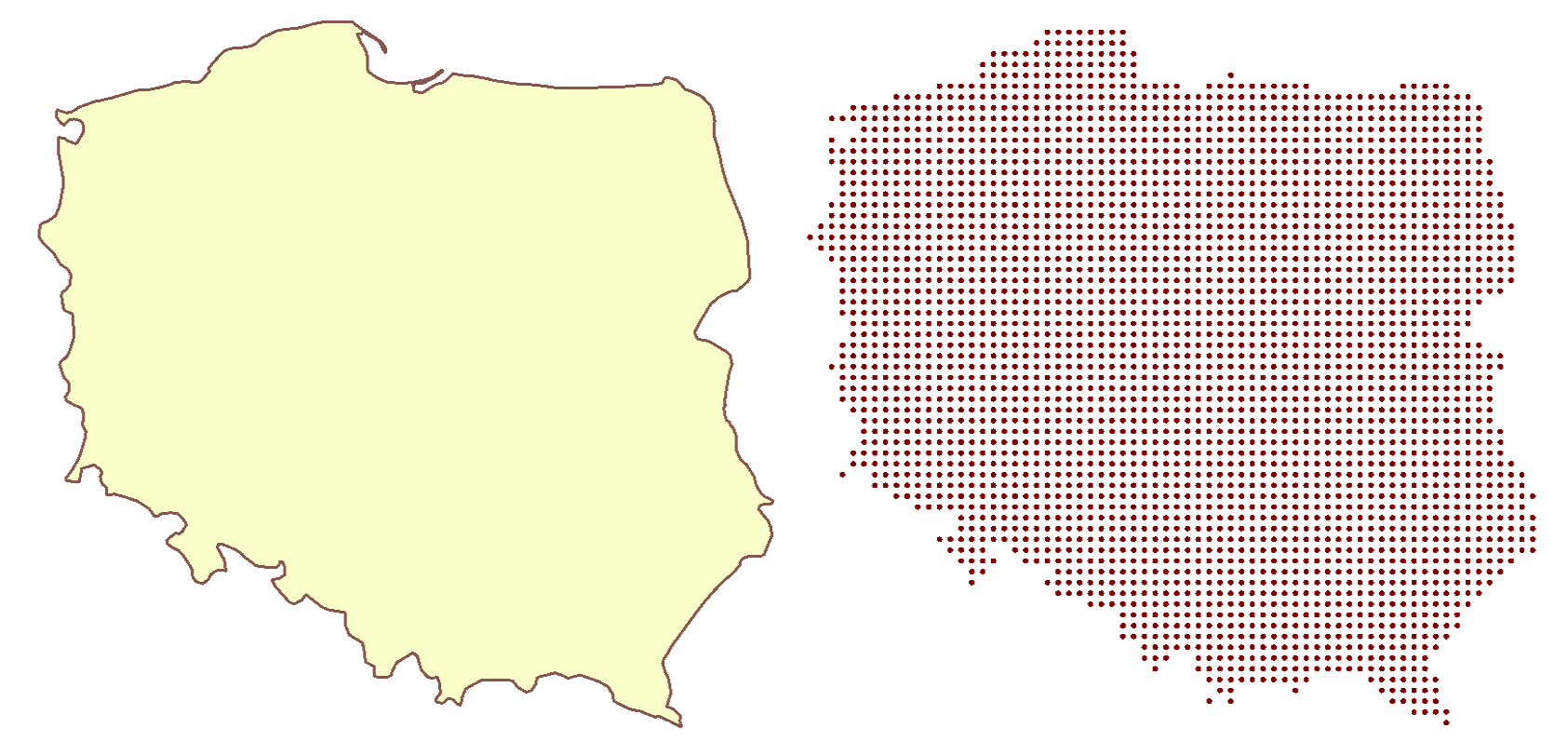
First, turn a polygon into an evenly spaced point cloud.
FME also can, with PointCloudCoercer, split point clouds into multipoints with a preset number of points. Considering the equal spaces between points and the equal number of points in the multipoints, we can assume that the pieces we get from PointCloudCoercer occupy areas of approximately the same size:

Then split the point cloud into multipoints of approximately equal size.
Now if we can turn these multipoints into polygons, we have the solution. The problem is, the multipoints have thin gaps between each other because points themselves have no size.

Before turning the multipoint geometries into polygons, resolve the gaps between them.
In my original workspace made in 2013, I used HullReplacer to get concave hulls, which then I tried to clean with a lot of vector transformers, which included Generalizer, AnchoredSnapper, CenterlineReplacer, etc. That was the weakest part of the workflow – slow, and the quality of the vector output was not great at all.
While I was working on this article, I decided to re-evaluate my approach to polygon creation, and found a more elegant solution, which also involves more geometry types – I decided to rasterize the multipoints. Raster cells always have some size, and if we set that size to the spacing used for making the point cloud, we will fill all the gaps between the pieces.
Depending on the splitting mode, we can get different results. “Spatial Equal Points Multipoints” mode produces areas with less variation in their sizes, and “Nested Equal Area Multipoints” makes better shapes.

Tiled polygon results from two different splitting modes.
Viewshed Analysis
Viewshed analysis is a common function of many GIS packages. It determines visibility from/to a certain point to/from the cells of a DEM (Digital Elevation Model) raster.

How viewshed analysis works. (Credit: Zoran Čučković)
FME does not have a specific transformer to perform such analysis. Mike Oberdries from Oberdries Consulting Ltd, New Zealand, asked me about a possibility of doing viewshed analysis with FME, luring me into it by saying this was a “Dmitri-type” question. Am I revealing too much about myself?
After initially saying “No”, I kept thinking how I could approach the problem, and again, decided to give a try to a point cloud technique. Within a few days I came up with an idea, which was successfully implemented and helped us to break a few FME world records – during the transformation, which took about 24 hours, we had to deal with 17,000,000,000 points.
Mike’s scenario is pretty specific to his dataset; this is why here I am going to show a more general approach to the problem.
At the beginning, we only have a raster DEM and a point representing the location of the observer.

The two inputs to a viewshed analysis problem.
We generate a unique ID for each raster cell (target) and make a point cloud from the DEM with PointCloudCombiner, in which each pixel becomes a point with XYZ coordinates and the cell ID as a component.
In the next step, we measure the distance between the observer and the target points (using simple Pythagorean theorem – my algorithm does not take the curvature of the Earth into account), and make visibility rays as sets of points along the imaginary 3D lines connecting the observer and the targets. So, for example, if the distance is 100 meters, and we decided that the point density of our rays should be 5 meters, we will get 20 points between the observer and the target.
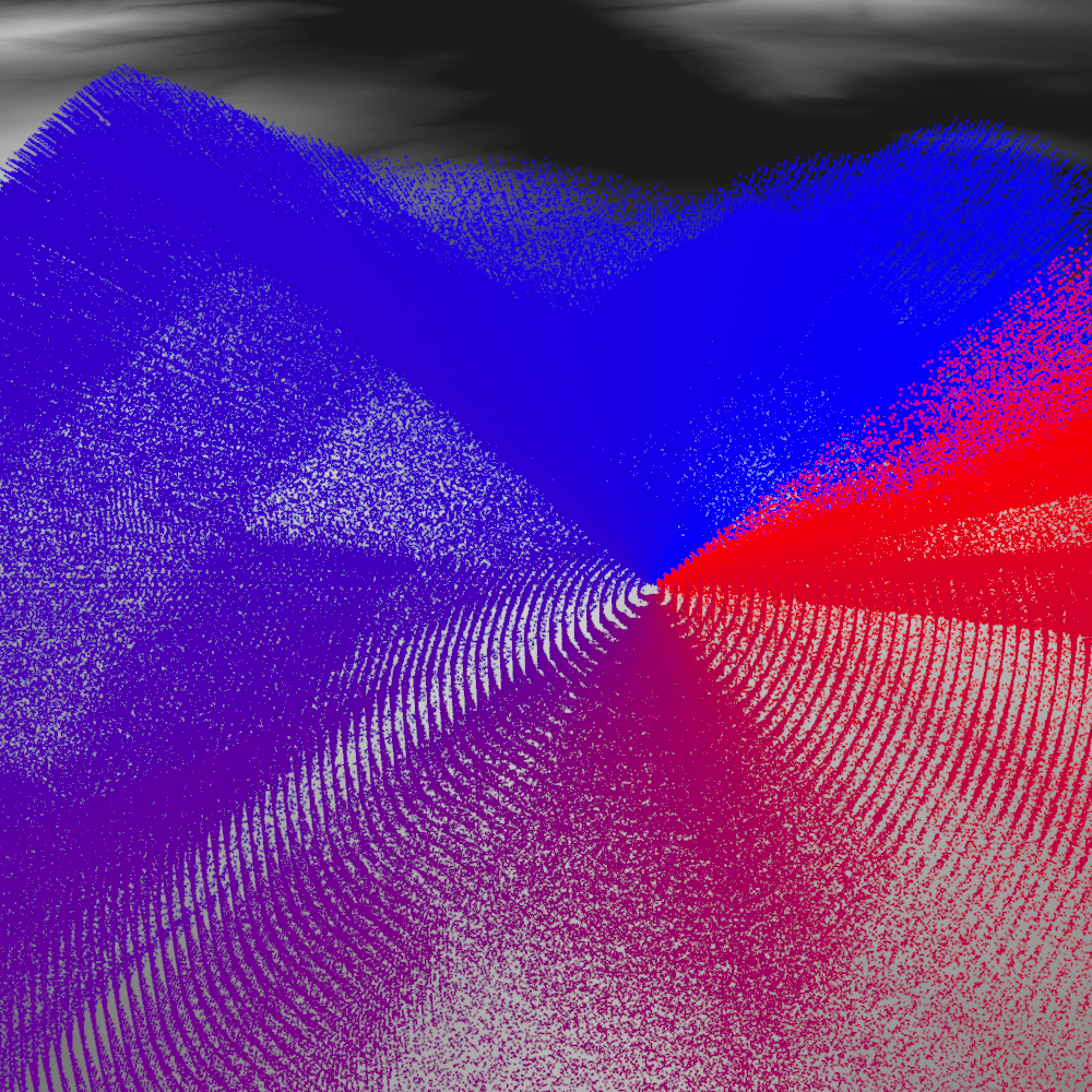
The observer’s visibility, represented as points along lines.
Once we have all the points, we overlay them with the DEM using PointCloudOnRasterComponentSetter. Each point will receive the ground elevation at its location. Now we can easily split the point cloud into two with PointCloudFilter by comparing the difference between the point and ground elevations. If the difference is bigger than or equal to 0, the point is above or on the ground, otherwise, it is below the ground.
So, by this moment, each point “knows” whether it is above or below the ground, and to which ray it belongs. This means from now on we don’t need X, Y, and Z in this point cloud – we can remove these components for faster processing (PointCloudComponentRemover) – and keep only one component, which is the ray ID.
We can take only the point cloud with points below the ground, and merge it with itself (PointCloudMerger) by ray ID. If we use only the output from the Referenced port, we get a single point per ray. Essentially, this is a list of rays having points (or cells) not visible by the observer. We can compare this point cloud with the original point cloud (which has XYZ) and for the rays with no match, we have a full visibility, that is, all the points of the ray are above the ground.
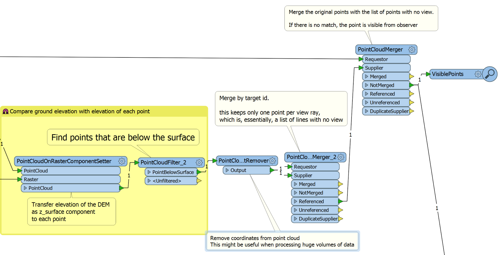
FME Workspace that overlays the DEM on the visibility ray point cloud and outputs the visible points.
After that we can, for example, rasterize the results (ImageRasterizer), generate a surface (TINGenerator) from the original DEM and apply the raster as a texture onto the surface (SharedItemAdder and SharedItemIDSetter).
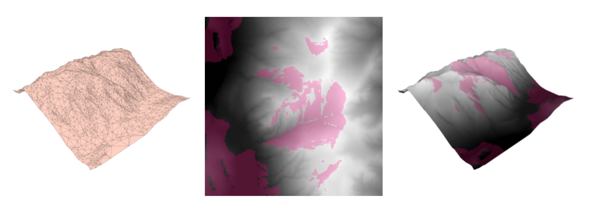
Generating a surface model and a raster, and overlaying them to provide a useful output.
If we generate a series of rasters changing the elevation of the observer, we can even get a nice animated GIF:
Viewshed analysis as an animated GIF.
Raster Coloring
We have had quite a few requests asking for raster coloring functionality. We have a custom transformer RasterHSVShader created by Jens Frolik available through FME Hub, which makes a colored hillshaded representation of a DEM using the HSV (hue, saturation, value) model. We also have a very powerful RasterExpressionEvaluator that can change pixel colors any way we want, but applying even a simple color ramp may require creating an outrageously complicated condition.
During the FME World Tour 2016, I got another request for coloring DEM rasters represented in FME with the boring grayscale tones and decided to tackle this problem. How great it would be to just take a predefined color ramp and apply it to any DEM. For testing purposes, I created such a ramp in the form of an RGB raster in Paint.Net.

Color ramp as an RGB raster.
How can we spread these colors along the range of DEM elevations? The answer should be already obvious – with a point cloud!
We turn the original raster into a point cloud, copy the XYZ values into the temporary components (x_orig, y_orig, z_orig), and set the new XYZ values:
- X is 0.
- Y is set to Z, so we get a point cloud consisting of points along a straight line, going from lowest to highest elevation values along the Y axis.
- Z is irrelevant, and may be set to any value, not set at all, or even removed.
The color ramp raster also needs some transformation before we can borrow its colors. We resample the color ramp so that along the Y axis, it has a pixel for every integer value in the elevation range. Then we georeference the ramp so that it gets placed along the points of our DEM point cloud, which is currently, as the paragraph above explains, just set of points along a line:
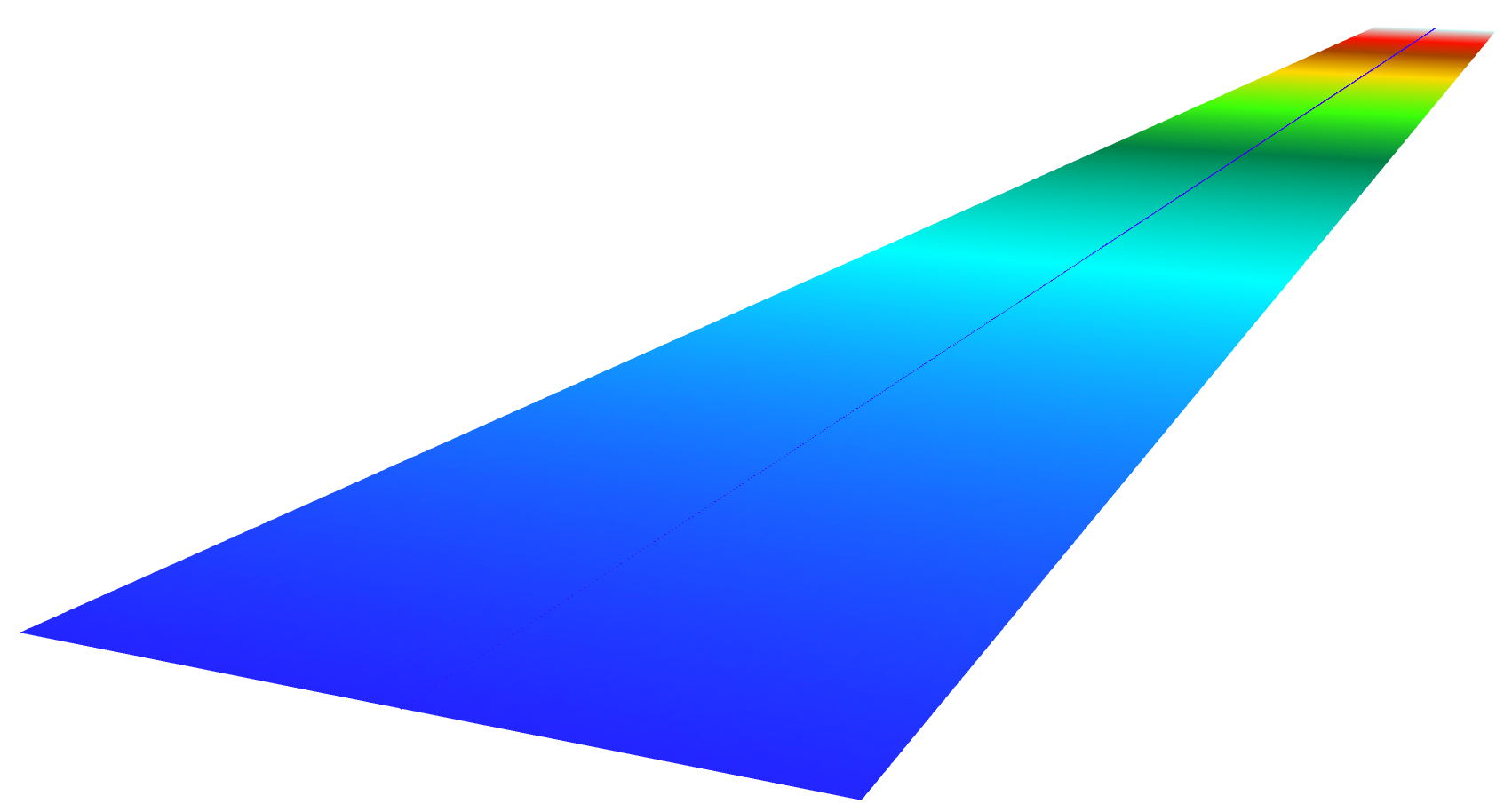
The original raster becomes an elevation-sorted point cloud (the line up the middle), and the color ramp is placed along it.
PointCloudOnRasterComponentSetter brings RGB values from the ramp to the points of the DEM, and PointCloudComponentCopier restores the original XYZ values. Now if we rasterize our point cloud, we will get a nicely colored RGB raster (the original is on the left along with the color ramp, the result of the coloring is on the right):
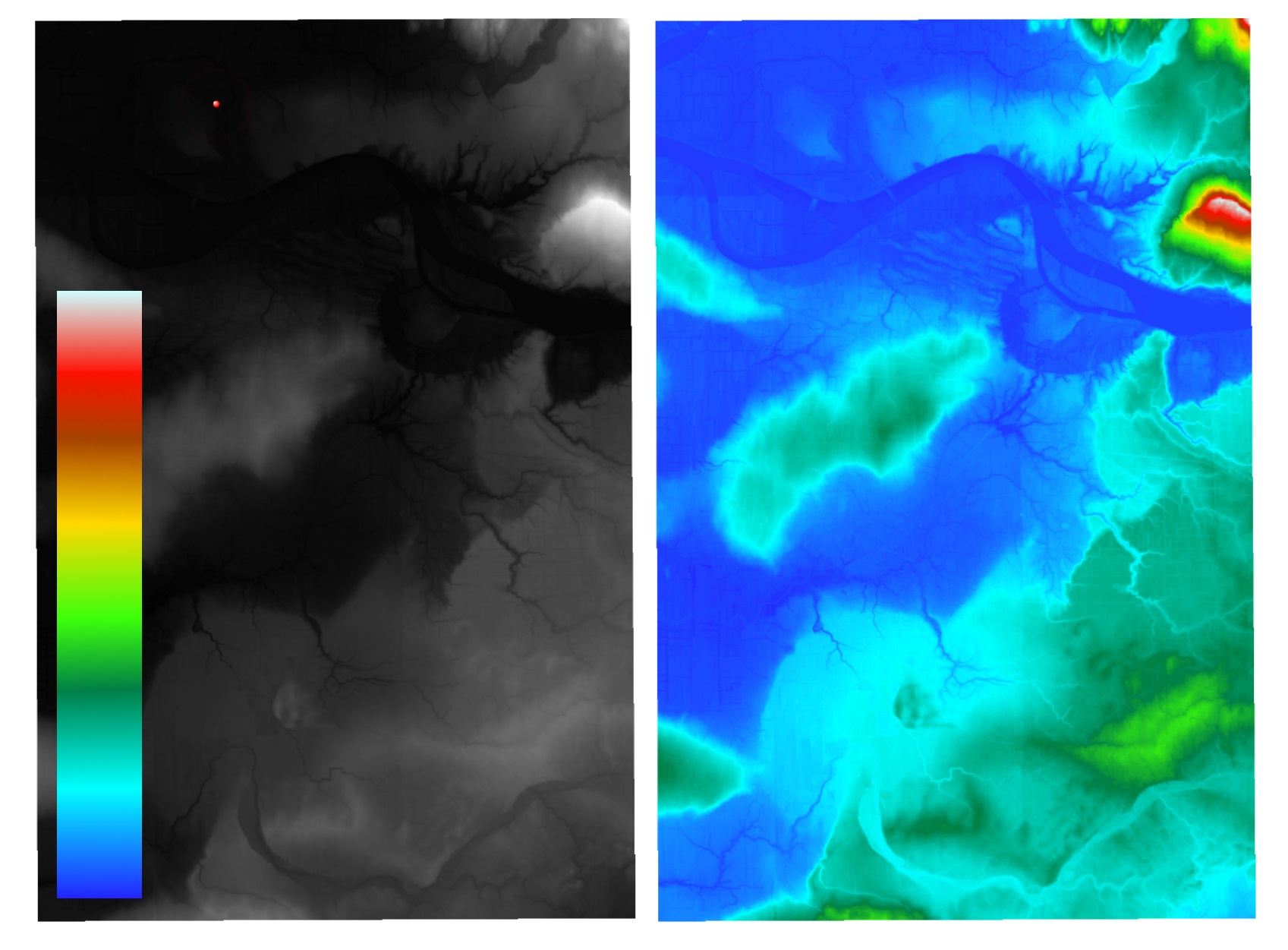
Original raster and color ramp (left) and colorized result (right).
Using this technique means that the color ramp does not necessarily have to look as a traditional stripe with gradually changing colors – we can use ANY image to color the raster and get some stunningly beautiful images that resemble agate-like patterns.
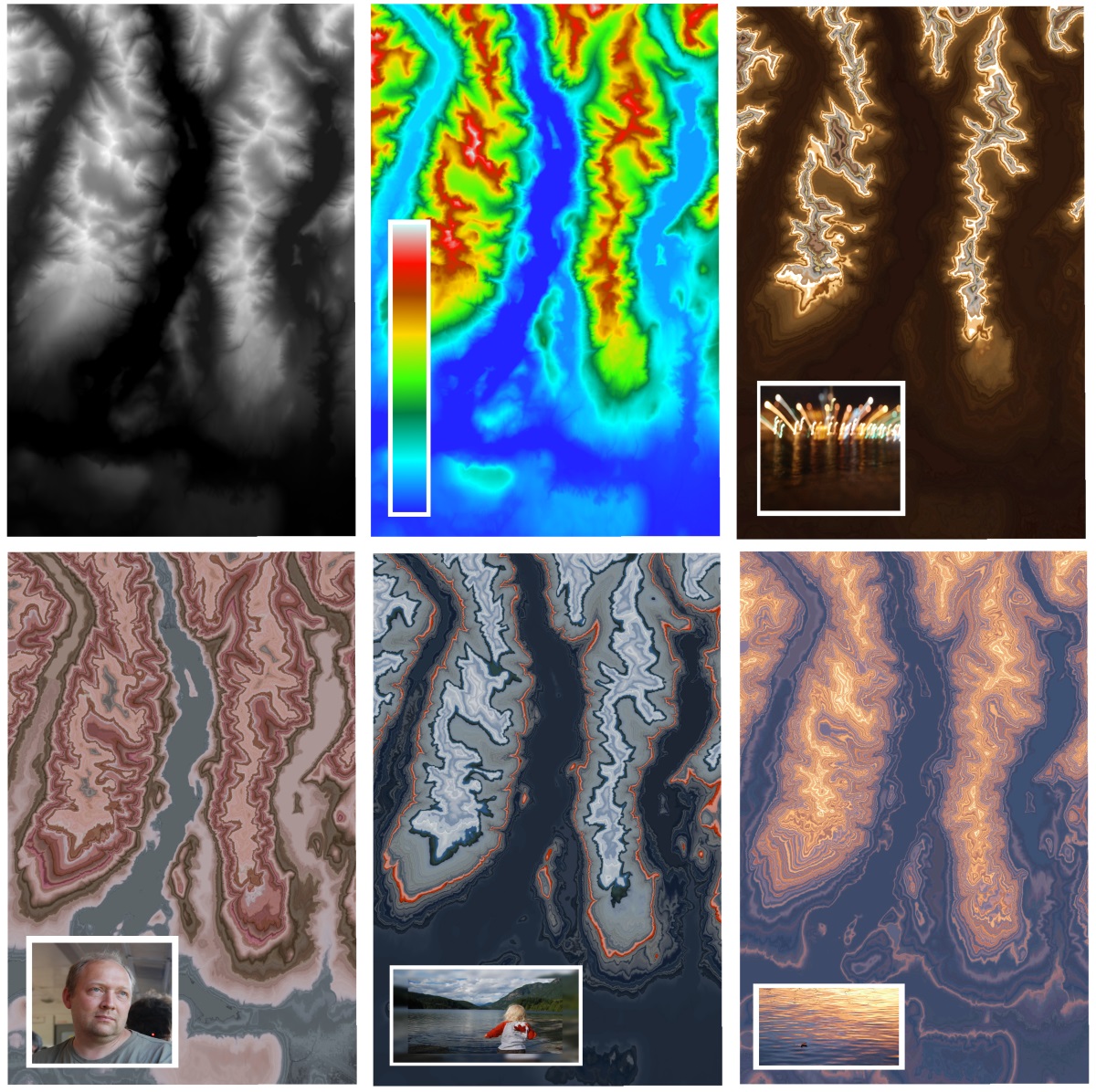
Original raster (top left) and several outputs using various images as a color ramp.
Raster Statistics
Another frequent request is RasterStatisticsCalculator. Unfortunately, as of May 2016, FME does not have such a transformer. It is very easy to get around it because, as it was shown above, we can turn the raster into a point cloud, and for this geometry we have PointCloudStatisticsCalculator.
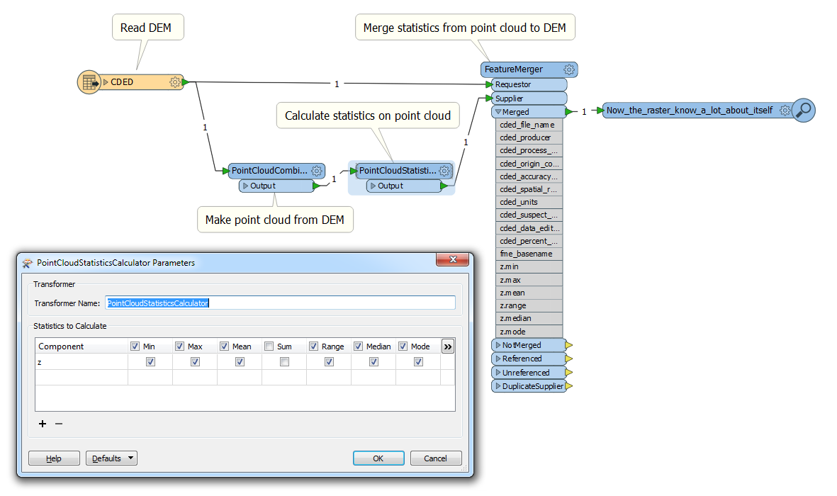
Calculating raster statistics using FME’s PointCloudStatisticsCalculator.
Once the statistics are calculated, we can merge the statistical attributes back with the original raster or process them separately.
Conclusion
I really hope my examples showed how powerful point cloud techniques can be when they are applied outside of their traditional domain.
The potential to fully restructure the geometric representation of a point cloud and restore it to its original look is a great method of comparing and analyzing different datasets.
Plus, the ability to go between different geometry types allows us to choose the best geometry for a particular operation.
Finally, imagine if we could in the future apply the point cloud processing speed to regular vector features. Well, this bright future might be not that far away – we’re working hard to make it happen soon.
Should I suggest a slogan for the next FME World Tour: “Making a difference, one million features at a time”?

Dmitri Bagh
Dmitri is the scenario creation expert at Safe Software, which means he spends his days playing with FME and testing what amazing things it can do.